Reconstructing a Gaussian Splat Radiance Field and High Quality Mesh from a Capture
In this notebook, we’ll walk through how to reconstruct a Gaussian Splat radiance field, and high quality triangle mesh from an input drone capture. The capture consists of a collection of posed images along with sparse points. We’ll show how you can visualize this radiance field interactively in a notebook or browser, how to save the radiance field to common formats like PLY and USDZ, and how to use the radiance field to construct a high quality triangle mesh. Along the way, we’ll get a tour of the basic components of the fvdb_reality_capture library.
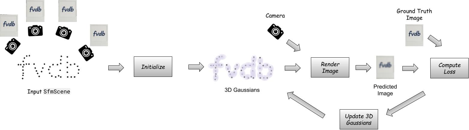
The notebook walks through a common reality capture pipeline like in the figure below:
Setup and imports
Before we get started, let’s import the pacakges we need. Here’s an overview of some of the important ones:
loggingWe’ll use the built-in Python
loggingmodule, and calllogging.basicConfig()which will cause functions withinfvdb_reality_captureto log to stdout. You don’t have to enable this, but it’s useful to see what’s happening under the hood.
fvdbWe use
fvdbfor the underlying Gaussian splat data structure (fvdb.GaussianSplat3d) which provides fast and scalable rendering, and for interactive visualization (using thefvdb.viz) module.
fvdb_reality_captureWe use this for core algorithms that reconstruct scenes from sensors help us read and process capture data (Duh!)
import logging

import cv2
import fvdb
import matplotlib.pyplot as plt
import numpy as np
import torch

import fvdb_reality_capture as frc

# Let's use verbose logging to track what happens under the hood.
# For less output set level=logging.WARN. For more set level=logging.DEBUG
logging.basicConfig(level=logging.INFO, format="%(levelname)s : %(message)s")

# Initialize the fvdb.viz module for interactive 3D visualization.
# This will spin up a small HTTP server in the background.
fvdb.viz.init(port=8080)
Viewer Info: Running in headless mode - no GLFW window created
Download some example data
Let’s download some example data to run on. We’ll use the “safety_park” example dataset. This dataset is the output of a COLMAP structure from motion pipeline on a sequence of images captured by a drone.
It contains posed images (i.e. images + the position and orientation of the camera that took them), camera intrinsic parameters (focal length, optical centers, etc.), and a set of sparse 3D points at known surfaces in the scene.
# Download example data for running splats on
frc.tools.download_example_data(dataset="safety_park", download_path="./data")
Viewer Info: Server created on port(8080)
Viewer Info: Running on server 127.0.0.1:8080


2025-10-19 17:35:13,310 - fvdb_reality_capture.tools._download_example_data.download_example_data - INFO - Downloading dataset safety_park from https://fvdb-data.s3.us-east-2.amazonaws.com/fvdb-reality-capture/safety_park.zip to data/safety_park/safety_park.zip
Downloading dataset safety_park: 100%|██████████| 1.05G/1.05G [00:50<00:00, 21.0MB/s]
2025-10-19 17:36:03,335 - fvdb_reality_capture.tools._download_example_data.download_example_data - INFO - Dataset downloaded successfully.
2025-10-19 17:36:03,335 - fvdb_reality_capture.tools._download_example_data.download_example_data - INFO - Extracting archive safety_park.zip to data/safety_park.
Load our dataset into an SfmScene for reconstruction
Reality capture is the process of creating digital 3D representations of real-world scenes from sensor data, like images and LiDAR. To represent captured sensor data, fvdb_reality_capture makes use of the SfmScene class, which is a lightweight handle to sensor data stored on disk. SfmScene offers a wide range of features for efficiently transforming large-scale datasets, some of which we’ll see below. For a detailed tutorial, see the Loading and Manipulating Sensor Data tutorial.
An SfmScene consists of the following parts representing a scene captured with sensors:
A list of Posed images.
Images with camera-to-world/world-to-camera transformations specifying where each image was taken in the scene, and the identifier of the camera that captured them.
A set of Camera sensors.
Information such as camera intrinsics and distortion parameters for each camera used to capture the scene.
Note the number of cameras is not the same as the number of posed images. If you captured 1000 images with a robot that had two cameras, there will be two cameras and 1000 posed images
A set of Scanned 3D points
These are points for which we have high confidence lie on a surface in the scene.
An (optional) Point visibility map
These define the set of points visible within each posed image.
This type of sensor data may arise from capture hardware (e.g. a set of cameras and LiDAR sensors equipped with Inertial Measurement Units (IMU) sensors), or from Structure-from-Motion (Sfm) capture which solves for camera poses and points using correspondences between a set of images. fvdb_reality_capture aims to support loading a wide variety of capture data formats into an SfmScene.
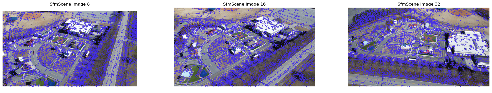
Let’s load our downloaded dataset into an SfmScene and visualize it. We’ll visualize the 3D points and cameras interactively using fvdb.viz and we’ll plot some images with their visible points using matplotlib. The fvdb.viz module provides a high performance debug visualizer written in vulkan. It spins up a small HTTP server which streams a visualization to a notebook or a browser.
dataset_path = "./data/safety_park"
sfm_scene = frc.sfm_scene.SfmScene.from_colmap(dataset_path)

# Visualize an image in an SfmScene and the 3D points visible from that images
# projected onto the image plane as blue dots.
def plot_image_from_scene(scene: frc.sfm_scene.SfmScene, image_id: int):
    image_meta: frc.sfm_scene.SfmPosedImageMetadata = scene.images[image_id]
    camera_meta: frc.sfm_scene.SfmCameraMetadata = image_meta.camera_metadata

    # Get the visible 3d points for this image
    visible_points_3d: np.ndarray = scene.points[image_meta.point_indices]

    # Project those points onto the image plane
    # 1. Get the world -> camera space transform and projection matrix
    world_to_cam_matrix: np.ndarray = image_meta.world_to_camera_matrix
    projection_matrix: np.ndarray = camera_meta.projection_matrix
    # 2. Transform world points to camera space
    visible_points_3d_cam_space = world_to_cam_matrix[:3,:3] @ visible_points_3d.T + world_to_cam_matrix[:3,3:4]
    # 3. Transform camera space coordinates to image space
    visible_points_2d = projection_matrix @ visible_points_3d_cam_space
    visible_points_2d /= visible_points_2d[2]

    # Load the image and convert to RGB (OpenCV uses BGR by default)
    loaded_image = cv2.imread(image_meta.image_path)
    assert loaded_image is not None, f"Failed to load image at {image_meta.image_path}"
    loaded_image = cv2.cvtColor(loaded_image, cv2.COLOR_BGR2RGB)

    # Plot the image and projected points
    plt.title(f"SfmScene Image {image_id}")
    plt.axis("off")
    plt.imshow(loaded_image)
    plt.scatter(visible_points_2d[0], visible_points_2d[1], color="#432de9", marker=".", s=2)

# Visualize the SfmScene interactively in a 3D viewer using fvdb.viz.Viewer
def visualize_sfm_scene(scene: frc.sfm_scene.SfmScene,
                        name: str,
                        center_scene: bool = False):

    viewer_scene = fvdb.viz.get_scene("SfmScene Visualization")
    # Optionally center the scene at the origin.
    # This is useful to visualize multiple scenes together without them being far apart.
    if center_scene:
        center_transform = np.eye(4)
        center_transform[:3, 3] = -np.median(scene.points, axis=0)
        scene = scene.apply_transformation_matrix(center_transform)

    # Plot the points in the SfmScene with their colors (which are uint8 by default but the viewer
    # expects float32 colors in [0,1]).
    # Each point is drawn as a small sphere with a 2 pixel radius.
    viewer_scene.add_point_cloud(
        name=f"{name} Points",
        points=scene.points,
        colors=scene.points_rgb.astype(np.float32) / 255.0,
        point_size=2.0)

    # Plot the cameras as coordinate frames with axis length 2 units,
    # and frustums whose distance from the origin to camera plane is 1 unit long.
    viewer_scene.add_cameras(
        f"{name} Cameras",
        camera_to_world_matrices=scene.camera_to_world_matrices,
        projection_matrices=scene.projection_matrices,
        axis_length=2,
        frustum_scale=2.5,
    )

    # Set the initial camera view to be at the position of the first posed image, in the SfmScene,
    # looking at the center of the 3D points, with Z as up (COLMAP SfM scenes use Z as up).
    viewer_scene.set_camera_lookat(
        eye=scene.image_camera_positions[0],
        center=np.zeros(3),
        up=np.array([0, 0, 1]),  # Z is up in COLMAP SfM scenes
    )


# Plot three images from the scene and their visible 3D points alongside each other
plt.figure(figsize=(25, 4.25))
plt.subplot(1, 3, 1)
plot_image_from_scene(sfm_scene, 8)
plt.subplot(1, 3, 2)
plot_image_from_scene(sfm_scene, 16)
plt.subplot(1, 3, 3)
plot_image_from_scene(sfm_scene, 32)
plt.show()

# View the SfmScene interactively in a 3D viewer
visualize_sfm_scene(sfm_scene, "Raw SfmScene", center_scene=True)
fvdb.viz.show()
2025-10-19 17:36:06,902 - fvdb_reality_capture.sfm_scene._load_colmap_scene.load_colmap_scene - INFO - Computing and caching visible points per image...
100%|██████████| 199702/199702 [00:01<00:00, 197220.05it/s]
You may have noticed the scene in the viewer is rotated with respect to the canonical axes. It’s also very noisy with a lot of outlier points. This is because the structure-from-motion algorithm which produced this data had a lot of noisy predictions, and predicted points and cameras in a rotated coordinate frame. Before we reconstruct a Gaussian Splat radiance field, let’s clean up our input data a bit. We’ll apply the following steps:
Downsample the images by a factor of 4 to speed up Gaussian Splat optimization (loading big images can be time consuming),
Normalize the scene to a canonical coordinte space by rotating it to align with the principle axes of the point cloud (thus correcting the up-axis).
Remove outlier points below the bottom 3rd and above top 97th percentiles along the X, Y, and Z, axis.
Remove any images with fewer than 50 visible points (these images are likely to have bad pose estimates)
fvdb_reality_capture makes this kind of cleanup easy, efficient, and seamless using the transforms module.
Transforms are classes which define a transformation of an SfmScene. They inherit from fvdb_reality_capture.BaseTransform, and their __call__ operator accepts an SfmScene as input and produces a new SfmScene as output. Let’s look at some code and visualizations and then dive into how this works.
import fvdb_reality_capture.transforms as fvtransforms

# Clean up and resize the SfmScene using a transform pipeline which downsamples images,
# aligns the scene with its principle axes and centers it at (0, 0, 0),
# filters outlier points, and removes images with too few points.
cleanup_and_resize_transform = fvtransforms.Compose(
    fvtransforms.DownsampleImages(image_downsample_factor=4, image_type="jpg", rescaled_jpeg_quality=95),
    fvtransforms.NormalizeScene(normalization_type="pca"),
    fvtransforms.PercentileFilterPoints(percentile_min=3.0, percentile_max=97.0),
    fvtransforms.FilterImagesWithLowPoints(min_num_points=50),
)
cleaned_sfm_scene = cleanup_and_resize_transform(sfm_scene)

print(f"Original scene had {len(sfm_scene.points)} points and {len(sfm_scene.images)} images")
print(f"Cleaned scene has {len(cleaned_sfm_scene.points)} points and {len(cleaned_sfm_scene.images)} images")

# Visualize the transformed scene so we can see the effect of the cleanup and resizing
# Note that we don't have to center the scene here since the normalization transform already did that.
visualize_sfm_scene(cleaned_sfm_scene, "Cleaned SfmScene", center_scene=False)
2025-10-19 17:36:09,105 - fvdb_reality_capture.transforms.downsample_images.DownsampleImages - INFO - Rescaling images using downsample factor 4, sampling mode 3, and quality 95.
2025-10-19 17:36:09,106 - fvdb_reality_capture.transforms.downsample_images.DownsampleImages - INFO - Attempting to load downsampled images from cache.
2025-10-19 17:36:09,106 - fvdb_reality_capture.transforms.downsample_images.DownsampleImages - INFO - No downsampled images found in the cache.
2025-10-19 17:36:09,107 - fvdb_reality_capture.transforms.downsample_images.DownsampleImages - INFO - Generating images downsampled by a factor of 4 and saving to cache.
Rescaling 000079.jpg from 3840 x 2160 to 960 x 540:  16%|█▌        | 20/124 [00:01<00:06, 15.25imgs/s]

Rescaling 000182.jpg from 3840 x 2160 to 960 x 540: 100%|██████████| 124/124 [00:08<00:00, 15.42imgs/s]
2025-10-19 17:36:17,148 - fvdb_reality_capture.transforms.downsample_images.DownsampleImages - INFO - Rescaled 124 images by a factor of 4 and saved to cache with sampling mode 3 and quality 95.
2025-10-19 17:36:17,148 - fvdb_reality_capture.transforms.normalize_scene.NormalizeScene - INFO - Normalizing SfmScene with normalization type: pca
2025-10-19 17:36:17,161 - fvdb_reality_capture.transforms.percentile_filter_points.PercentileFilterPoints - INFO - Filtering points based on percentiles: min=[3. 3. 3.], max=[97. 97. 97.]


Original scene had 199702 points and 124 images
Cleaned scene has 168661 points and 124 images
Note how the cleaned up scene has fewer noisy points and is aligned with the coordinate axes of the viewer.
In the code above, we defined our cleanup operation as a sequence of transformations, using the Compose transform, which composes a sequence of transforms into a single one. The composed transform runs the following in order:
DownsampleImages(4)to downsample each image in the dataset by a factor of 4NormalizeScene('pca')to center the scene about its mean and rotate it to align with its principle axes.PercentileFilterPoints(percentile_min=3.0, percentile_max=97.0)to remove points in the bottom 3rd and top 97th percentiles along each axis.FilterImagesWithLowPoints(min_num_points=50)to remove posed images which have 50 or viewer visible points.
Note: fvdb_reality_capture provides more transforms and also lets you define your own transforms. See the API reference for fvdb_reality_capture.transforms and the the Loading and Manipulating Sensor Data tutorial for more details.
Note: The fvdb_reality_capture.transforms module does not modify the underlying dataset that you pass in or store transformed data in memory.
Instead, it uses a cache which lets each transform cache intermediate results. This keeps SfmScenes lightweight and immutable, and
lets you transform your data in a clean and non-destructive way.
To see the caching in action, remark how the first transformation took a while. If we run the process again, it’s almost instantaneous due to caching.
# The transform pipeline caches results so re-applying it is very fast
%time cleaned_sfm_scene = cleanup_and_resize_transform(sfm_scene)
2025-10-19 17:36:17,366 - fvdb_reality_capture.transforms.downsample_images.DownsampleImages - INFO - Rescaling images using downsample factor 4, sampling mode 3, and quality 95.
2025-10-19 17:36:17,366 - fvdb_reality_capture.transforms.downsample_images.DownsampleImages - INFO - Attempting to load downsampled images from cache.
2025-10-19 17:36:17,396 - fvdb_reality_capture.transforms.normalize_scene.NormalizeScene - INFO - Normalizing SfmScene with normalization type: pca
2025-10-19 17:36:17,399 - fvdb_reality_capture.transforms.percentile_filter_points.PercentileFilterPoints - INFO - Filtering points based on percentiles: min=[3. 3. 3.], max=[97. 97. 97.]


CPU times: user 471 ms, sys: 10.8 ms, total: 481 ms
Wall time: 179 ms
Reconstruct a Gaussian splat radiance field
A radiance field is a 3D scene representation that specifies the color of a point along a given view direction. Radiance fields enable high fidelity visualization of 3D captures with realistic lighting effects.
3D Gaussian Splatting1 is the dominant radiance field representation. 3D Gaussian splats encode a radiance field function as a sum of Gaussians, parameterized by their means (positions), rotations, and scales. Additionally each Gaussian has an opacity value and a set of spherical harmonics that map the direction in which a Gaussian is viewed to a color.
fvdb_reality_capture provides tools to reconstruct a 3D Gaussian Splat radiance field from an SfmScene using the optimized GaussianSplat3d data structure in the fvdb-core library. The resulting reconstruction algorithm is robust, performant, and production-ready.
At a high level, reconstructing an fvdb.GaussianSplat3d from an SfmScene works as follows as follows. We initialize a set of 3D Gaussians directly using the SfmScene’s points. Then, we iteratively optimize the Gaussians in in two steps: First, we render images from the Gaussian splat by volume rendering the 3D gaussians using the algorithm first proposed in [1]. Second, we calculate a loss between the rendered images from the Gaussian Splat and the ground truth images in the SfmScene. Finally, we update the Gaussian’s parameters to reduce this loss via gradient descent. During this optimization, we periodically add new Gaussians to capture regions with high detail, and remove Gaussians in regions of low detail. The figure below illustrates this procedure pictorially.
The core API for Gaussian Splat reconstruction is the fvdb_reality_capture.GaussianSplatReconstruction class. It accepts an input SfmScene and optional config parameters, and produces an fvdb.GaussianSplat3d reconstructing the scene. Let’s see how to use it below to reconstruct a Gaussian splat radiance field from our cleaned up scene.
# We'll just reconstruct our scene using the default settings, which are good in most cases.
# See the documentation for `frc.GaussianSplatReconstruction` for details on the available options.
# Note that this process can take a while depending on the size of your scene.
runner = frc.radiance_fields.GaussianSplatReconstruction.from_sfm_scene(cleaned_sfm_scene)
runner.optimize()
2025-10-19 17:36:17,549 - fvdb_reality_capture.radiance_fields.gaussian_splat_reconstruction.GaussianSplatReconstruction - INFO - Created training and validation datasets with 124 training images and 0 validation images.
2025-10-19 17:36:17,873 - fvdb_reality_capture.radiance_fields.gaussian_splat_reconstruction.GaussianSplatReconstruction - INFO - Model initialized with 168,661 Gaussians
Gaussian Splat Reconstruction:   0%|          | 0/24800 [00:00<?, ?steps/s]2025-10-19 17:36:18,474 - fvdb_reality_capture.radiance_fields.gaussian_splat_reconstruction.GaussianSplatReconstruction - INFO - Starting to optimize camera poses at step 0 (epoch 0)
loss=0.095| sh degree=3| num gaussians=1,208,652:  20%|█▉        | 4959/24800 [00:48<04:22, 75.63steps/s]2025-10-19 17:37:06,552 - fvdb_reality_capture.radiance_fields.gaussian_splat_reconstruction.GaussianSplatReconstruction - INFO - Saving checkpoint at global step 4960.
loss=0.021| sh degree=3| num gaussians=1,552,032: 100%|█████████▉| 24799/24800 [06:32<00:00, 58.20steps/s]2025-10-19 17:42:50,747 - fvdb_reality_capture.radiance_fields.gaussian_splat_reconstruction.GaussianSplatReconstruction - INFO - Saving checkpoint at global step 24800.
2025-10-19 17:42:50,829 - fvdb_reality_capture.radiance_fields.gaussian_splat_reconstruction.GaussianSplatReconstruction - INFO - Training completed.
loss=0.021| sh degree=3| num gaussians=1,552,032: 100%|██████████| 24800/24800 [06:32<00:00, 63.16steps/s]
Visualize a Gaussian splat radiance field with fvdb.viz
A major benefit of a 3D radiance fields is that we can render them continuously from any point in space in real time. Let’s interactively visualize the reconstructed Gaussian Splat, examining the result from novel, freeform viewpoints. The viewer in fvdb.viz makes this straightforward by letting us visualize fvdb.GaussianSplat3d objects directly.
# Get the trained splat model from the reconstruction runner
model: fvdb.GaussianSplat3d = runner.model
# model, metadata = fvdb.GaussianSplat3d.from_ply("./reconstructed_model.ply")

# Clear previous contents from the viewer
# viewer.clear()

# Add our splat model to the viewer
scene = fvdb.viz.get_scene("Gaussian Splat Model Visualization")
scene.add_gaussian_splat_3d("Reconstructed Gaussian Splat Radiance Field", model)

scene.add_cameras(
    "Input Cameras",
    camera_to_world_matrices=cleaned_sfm_scene.camera_to_world_matrices,
    projection_matrices=cleaned_sfm_scene.projection_matrices,
    axis_length=2,
    frustum_scale=2.5,
)

# Set up the viewer's initial camera to be positioned at the first camera in the SfmScene
# looking at the center of the scene. This should give a good initial view of the model.
camera_position = cleaned_sfm_scene.images[0].origin
camera_lookat_point = model.means.mean(dim=0)
scene.set_camera_lookat(eye=camera_position, center=camera_lookat_point, up=(0, 0, 1)) # Colmap uses Z as up
fvdb.viz.show()
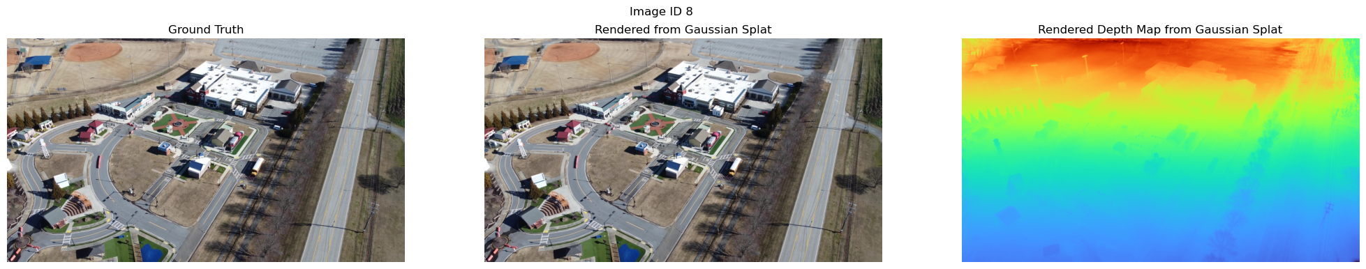
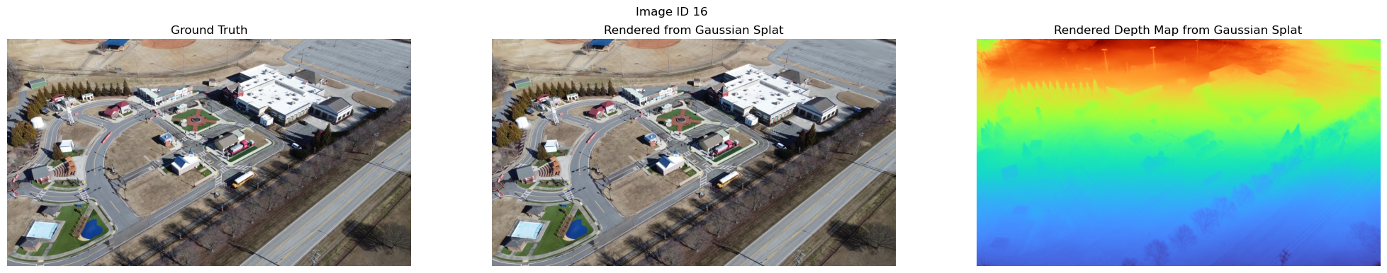
Plot images and depth maps from a Gaussian Splat radiance field
The GaussianSplatReconstruction class produces an fvdb.GaussianSplat3d object which encodes the radiance field. The fvdb.GaussianSplat3d class encodes a Gaussian splat radiance field and supports standard operations such as rendering images, depth maps, exporting to PLY, etc.
Let’s see how to use this class directly to plot some re-rendered images from the optimed Gaussian splat and compare them to their ground truth counterparts. We’ll also plot depth maps to visually inspect if the geometry of our reconstructed radiance field makes sense.
@torch.no_grad()
def plot_reconstruction_results(model: fvdb.GaussianSplat3d, sfm_scene: frc.sfm_scene.SfmScene, image_id: int):
    # Get one of the images and its camera from the scene
    image_meta: frc.sfm_scene.SfmPosedImageMetadata = sfm_scene.images[image_id]
    camera_meta: frc.sfm_scene.SfmCameraMetadata = image_meta.camera_metadata
    camera_to_world_matrix = torch.from_numpy(image_meta.camera_to_world_matrix).to(device=model.device, dtype=torch.float32)
    projection_matrix = torch.from_numpy(camera_meta.projection_matrix).to(device=model.device, dtype=torch.float32)
    image_height, image_width = image_meta.image_size

    # Read the ground truth image from disk
    gt_image = cv2.imread(image_meta.image_path)
    assert gt_image is not None, f"Failed to load image at {image_meta.image_path}"
    gt_image = cv2.cvtColor(gt_image, cv2.COLOR_BGR2RGB)

    # Render the image and a depth map from the Gaussian splat model
    rendered_rgbd, alphas = model.render_images_and_depths(
        world_to_camera_matrices=camera_to_world_matrix.inverse().unsqueeze(0).contiguous(),
        projection_matrices=projection_matrix.unsqueeze(0),
        image_width=image_width,
        image_height=image_height,
        near=0.1,
        far=10000.0,
    )
    rgb = rendered_rgbd[0, ..., :3].cpu().numpy()
    depth = (rendered_rgbd[0, ..., 3] / alphas.squeeze()).cpu().numpy()
    rendered_image = np.clip(rgb, 0.0, 1.0)
    rendered_image = (rendered_image * 255).astype(np.uint8)

    # Plot the ground truth and rendered images side by side
    plt.figure(figsize=(25, 4.25))
    plt.suptitle(f"Image ID {image_id}")
    plt.subplot(1, 3, 1)
    plt.title("Ground Truth")
    plt.axis("off")
    plt.imshow(gt_image)
    plt.subplot(1, 3, 2)
    plt.title("Rendered from Gaussian Splat")
    plt.axis("off")
    plt.imshow(rendered_image)
    plt.subplot(1, 3, 3)
    plt.title("Rendered Depth Map from Gaussian Splat")
    plt.axis("off")
    plt.imshow(depth, cmap="turbo")
    plt.show()

model: fvdb.GaussianSplat3d = runner.model
print(f"Reconstructed Gaussian Splat Model has {model.num_gaussians}, is on device {model.device}, and renders images with {model.num_channels} channels.")
plot_reconstruction_results(model, cleaned_sfm_scene, image_id=8)
plot_reconstruction_results(model, cleaned_sfm_scene, image_id=16)
Reconstructed Gaussian Splat Model has 1552032, is on device cuda:0, and renders images with 3 channels.
Export a Gaussian Splat radiance field to PLY and USDZ
You can save Gaussian Splat models to PLY and USDZ files using fvdb_reality_capture. This is useful for exporting your Gaussian Splats to be used in other applications, like SuperSplat, Blender with the 3DGS Addon, or NVIDIA’s Isaac Sim. Let’s see how to do this below.
Try going to supersplat.at and dragging the PLY saved below to try it out.
from fvdb_reality_capture.tools import export_splats_to_usdz

# Save the model as a PLY file for viewing in external tools like SuperSplat
model.save_ply("reconstructed_model.ply", metadata=runner.reconstruction_metadata)

# Save the model as a USDZ file for viewing in tools like NVIDIA's Isaac Sim
export_splats_to_usdz(model, out_path="reconstructed_model.usdz")
2025-10-19 17:42:54,717 - fvdb_reality_capture.tools._export_splats_to_usdz - INFO - Creating USD file containing NuRec model
2025-10-19 17:42:54,775 - fvdb_reality_capture.tools._export_splats_to_usdz - INFO - Model bounding box: min=[-184.37056 -157.57402  -40.16857], max=[165.56892 198.76385  88.72124]
2025-10-19 17:42:54,985 - fvdb_reality_capture.tools._export_splats_to_usdz - INFO - USDZ file created successfully at reconstructed_model.usdz
Reconstruct a mesh from a Gaussian Splat radiance field
Our Gaussian splat model is capable of producing images and depths from novel views. A natural way to reconstruct a mesh from a Gaussian scene is by rendering depth maps from the camera poses used to reconstruct the model and fuse them into a truncated signed distance field (TSDF) using the TSDF fusion algorithm[2].
TSDF fusion accumulates noisy depth maps into a voxel grid, to approximate a signed distance field near the surface of the object. fvdb_reality_capture makes use of fvdb-core to provide a high performance implementation of TSDF integration on sparse voxels. This allows us to generate meshes from Gaussian splats at very high resolutions on the GPU while using minimal memory.
Let’s see how to reconstruct a mesh using the fvdb_reality_capture.tools module.
from fvdb_reality_capture.tools import mesh_from_splats
import point_cloud_utils as pcu

# The truncation margin determines the width of the narrow band around the surface in which we compute the TSDF.
# A larger margin will produce coarser voxels, while a smaller margin will produce finer voxels but may miss some surface details.
# Here we pick a truncation margin of 0.25 world units in our scene.
truncation_margin = 0.5

# This function returns a tensor of vertices, faces, and colors for the mesh.
# The vertices have shape (num_vertices, 3), the faces have shape (num_faces, 3),
# and the colors have shape (num_vertices, 3). The colors are in the range [0, 1].
v, f, c = mesh_from_splats(model, cleaned_sfm_scene.camera_to_world_matrices, cleaned_sfm_scene.projection_matrices, cleaned_sfm_scene.image_sizes, truncation_margin)

# Save the mesh as a PLY file for viewing in external tools using point_cloud_utils (https://fwilliams.info/point-cloud-utils/) [3]
pcu.save_mesh_vfc("reconstructed_mesh.ply", v.cpu().numpy(), f.cpu().numpy(), c.cpu().numpy())

print(f"Reconstructed mesh with {v.shape[0]:,} vertices and {f.shape[0]:,} faces")
Extracting TSDF:   0%|          | 0/124 [00:00<?, ?imgs/s, accumulated_voxels=2.53e+7]

Extracting TSDF: 100%|██████████| 124/124 [00:07<00:00, 16.14imgs/s, accumulated_voxels=1.48e+8]


Reconstructed mesh with 12,288,540 vertices and 19,493,229 faces
Note how the final voxel count for tsdf fusion was over 140 million! The sparse TSDF fusion in fvdb, can handle large voxel sizes.
If you open the saved mesh in your favorite editor you get something like this:
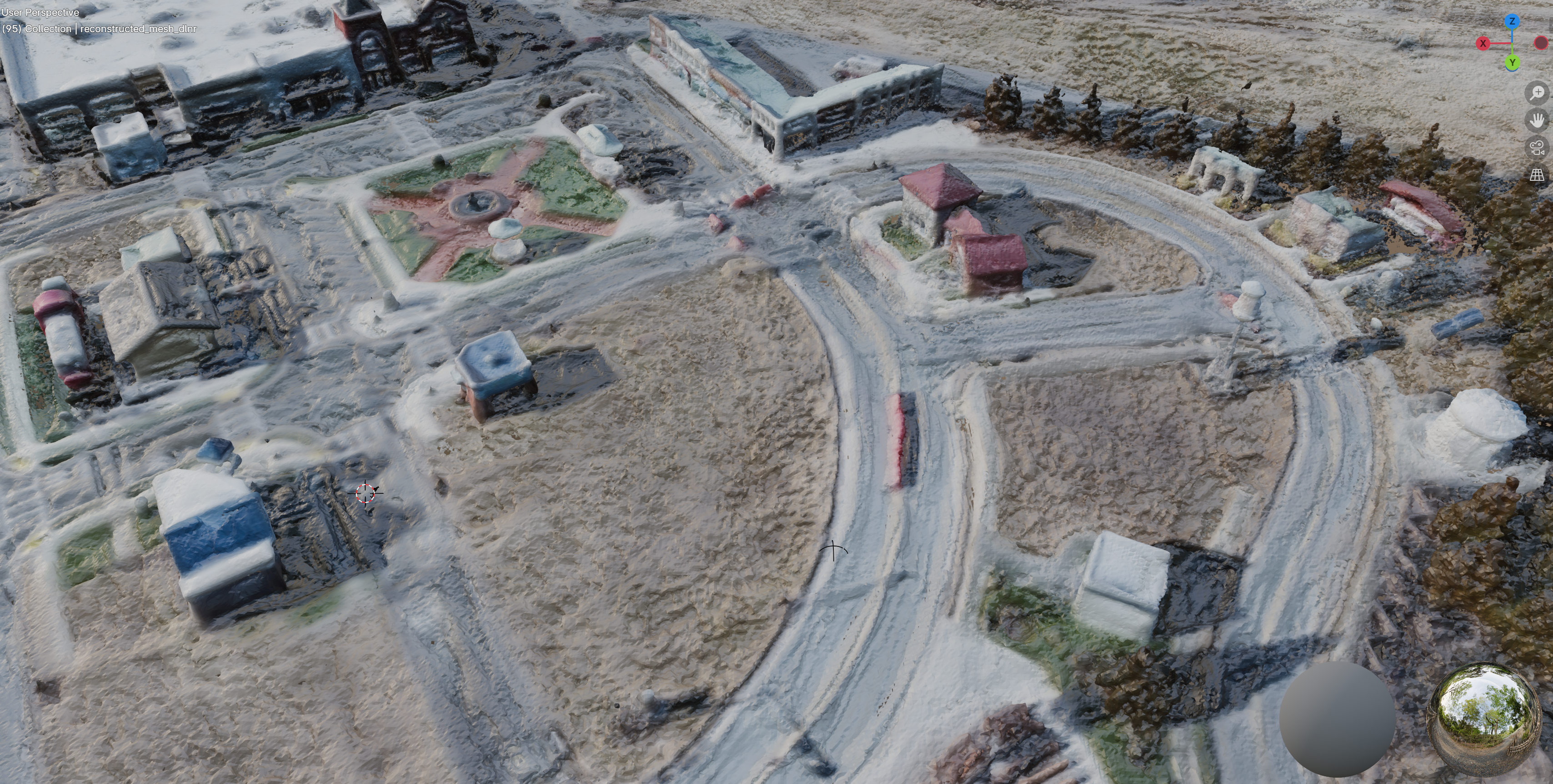
fvdb_reality_capture.tools provides a mesh_from_splats_dlnr which will use a foundation model to compute high quality depth maps from images rendered from our Gaussian splat.
The method works by rendering stereo pairs from the splat scene, and uses the DLNR foundation model[4] to perform stereo depth estimation. The DLNR model is a high-frequency stereo matching network that computes optical flow and disparity maps between two images
This method is generally slower to run since you have to evaluate a big neural network to estimate depth for each image, but produces much cleaner results.
Let’s see how to use this function to do mesh reconstruction:
from fvdb_reality_capture.tools import mesh_from_splats_dlnr
import point_cloud_utils as pcu

# The truncation margin determines the width of the narrow band around the surface in which we compute the TSDF.
# A larger margin will produce coarser voxels, while a smaller margin will produce finer voxels but may miss some surface details.
# Here we pick a truncation margin of 0.25 world units in our scene.
truncation_margin = 0.5

# This function has virtually the same interface as `mesh_from_splats`.
# It returns a tensor of vertices, faces, and colors for the mesh.
# The vertices have shape (num_vertices, 3), the faces have shape (num_faces, 3),
# and the colors have shape (num_vertices, 3). The colors are in the range [0, 1].
v, f, c = mesh_from_splats_dlnr(model, cleaned_sfm_scene.camera_to_world_matrices, cleaned_sfm_scene.projection_matrices, cleaned_sfm_scene.image_sizes, truncation_margin)

# Save the mesh as a PLY file for viewing in external tools using point_cloud_utils (https://fwilliams.info/point-cloud-utils/) [3]
pcu.save_mesh_vfc("reconstructed_mesh_dlnr.ply", v.cpu().numpy(), f.cpu().numpy(), c.cpu().numpy())

print(f"Reconstructed mesh with {v.shape[0]:,} vertices and {f.shape[0]:,} faces")
2025-10-19 17:43:05,507 - fvdb_reality_capture.foundation_models.dlnr.DLNRModel - INFO - Loading DLNR pretrained weights from /home/fwilliams/projects/openvdb/fvdb-reality-capture/fvdb_reality_capture/foundation_models/_weights/middlebury_dlnr.pth
2025-10-19 17:43:05,859 - fvdb_reality_capture.foundation_models.dlnr.DLNRModel - INFO - DLNR model loaded successfully.
Generating DLNR Depths:   0%|          | 0/124 [00:00<?, ?imgs/s]/home/fwilliams/bin/miniconda3/envs/fvdb/lib/python3.12/site-packages/torch/nn/functional.py:5096: UserWarning: Default grid_sample and affine_grid behavior has changed to align_corners=False since 1.3.0. Please specify align_corners=True if the old behavior is desired. See the documentation of grid_sample for details.
  warnings.warn(
Generating DLNR Depths: 100%|██████████| 124/124 [00:39<00:00,  3.14imgs/s]
Extracting TSDF: 100%|██████████| 124/124 [00:07<00:00, 16.88imgs/s, accumulated_voxels=5.98e+7]


Reconstructed mesh with 8,444,464 vertices and 14,809,696 faces
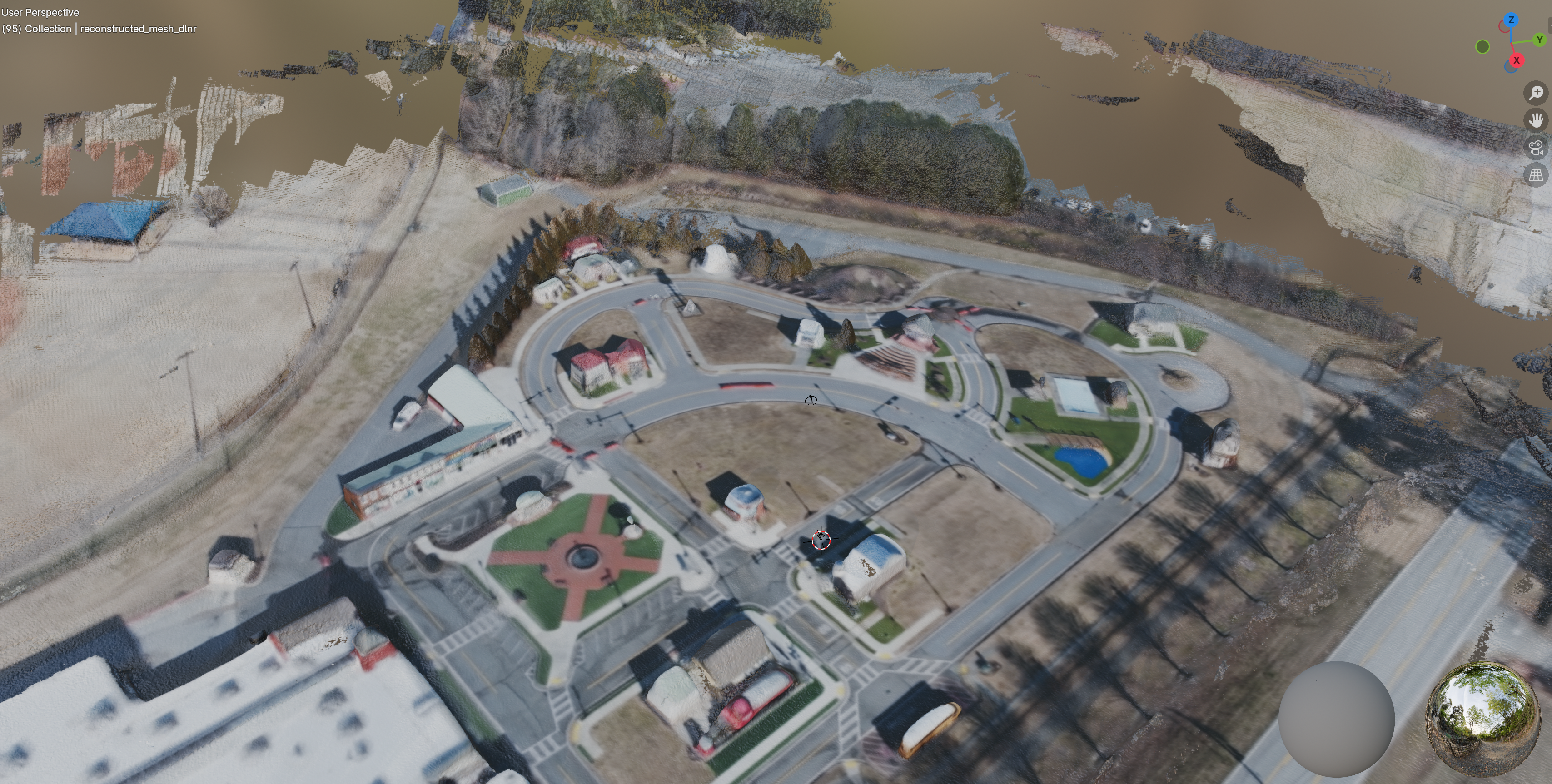
If you open the saved mesh in your favorite editor, you’ll see something like this. Much better!
Details are preserved, and there isn’t much noise in the reconstruction. In general, if you can afford the weight, you should stick to fvdb_reality_capture.tools.mesh_from_splats_dlnr for high quality mesh reconstructions.
References
[1] Kerbl, Kopanas et.al. - “3D Gaussian Splatting for Real-Time Radiance Field Rendering”
[2] Newcombe et.al. - “KinectFusion: Real-Time Dense Surface Mapping and Tracking”
[3] Williams - Point Cloud Utils
[4] Zhao, Zhou et.al. - High Frequency Stereo Matching